graphs | Mildly Interesting

The Weber-Fechner relations (from the 19th century) state that the neural representations in the brain of sensory stimuli, objects and time perception vary logarithmically with the intensity of the stimuli, the number of objects and the length of the time interval respectively.

Said mathematically, dP (change in perception) is proportional to dS/S (change in stimulus divided by stimulus magnitude) leading to P ~ O(ln S).

Some examples to illustrate what this means:

The higher the image resolution, the higher the delta further needed to make difference perceptible at all
The perceived costs/benefits of information production is proportional to the log of the amount of information that already exists (hence why we feel much more excited to work in green areas rather than beaten-up ones).

It so also happens that maximization of information content (entropy) under the above condition generates a power law distribution of the frequency and size of information when the information is dependent on one dimension (such as images that depend on resolution), or a log-normal distribution when the information is dependent on two dimensions (e.g., video/audio that depend on both resolution and time). This is explained in this paper.

Interestingly, if it were just the economic costs involved (and not the neurophysiological), then the distributions would be expected to be exponential, not power or lognormal.

Most symmetric social networks (such as Facebook, LinkedIn, IM) can be either viewed as directed graphs with bidirectional edges, or more simply as undirected graphs where two nodes connected by an undirected edge. A simple fact about random walks on such networks is the following:

Fact: A random walk on a finite, connected undirected graph with M edges has a stationary distribution π defined by $\pi_i = deg(i)/2M$ . This distribution is unique iff the graph is also aperiodic. An analogous result holds when the graph is weighted if we define $deg(i) = \sum_{j \leftrightarrow i} w_{ij}, W = \sum_i deg(i) \Rightarrow \pi_i = deg(i)/W$ .

This is interesting because instead of computing a very expensive random walk “simulation” (or doing matrix computations) to calculate the stationary distribution, we have a simple, closed formula. For example, the nodes can be “ranked” simply by their degree!

Background

A ‘random walk’ is a useful construct in graph algorithms. It is typically defined on a directed graph where the walk moves from a state i to a state j with probability p_ij. One such move or transition is sometimes called a step of the walk. Such a random walk is also known as a (homogeneous) Markov chain, which is a chain of random variables {X_j} such that Prob(walk is in node i after step j) = $Prob(X_j = i) = \sum_{k}Prob(X_{j-1}=k).p_{ki}$

Random walks have many applications in real-life networks. For example, the pagerank algorithm for scoring influence on the web and certain graph based social recommendation algorithms are essentially random walk algorithms.

A good background on random walks and Markov chains is in [1].

Proof

The proof is very simple. A distribution π is stationary if $\pi P = \pi$ where $P = (P_{ij})$ is the stochastic matrix defining the transition probability of going from state i to state j. Now, with a uniform random walk, each edge out of i can be taken with the same probability. i.e., $p_{ij} = 1/deg(i)$ . So,
$\pi_i = deg(i)/2M\\ \Rightarrow \pi_j = \sum_{k \leftrightarrow j} \pi_k.p_{kj} = \sum_k deg(k)/2M . 1/deg(k) = deg(j)/2M.$

A finite, connected graph is irreducible (every state can be reached from any other state). If the graph is aperiodic as well, the stationary vector is unique, and it is the normalized, eigenvector corresponding to the largest eigenvalue ( = 1 ) of the stochastic matrix P [1].

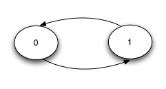
Real-life networks are certainly finite. They may not be connected or aperiodic, in which case care must be taken to artificially convert the graphs to be so. An example of an undirected graph with period 2 is simply the following graph.

Note that this can be made aperiodic by adding a self-edge from state 0 (or state 1) to itself.

Weighted Graphs

It turns out that the above mentioned fact remains true even when the undirected graph is weighted, i.e., each edge i ↔ j has a weight w_ij. The transition matrix is then defined by $p_{ij} = w_{ij}/W_i$ where $W_i = \sum_{j \leftrightarrow i}w_{ij}$ . Also, let $W = \sum_iW_i$ . The stationary vector is then defined by $\pi_i = W_i/W$ . The proof is very similar to the above.